
Lending Club Loan
Jifu Zhao, 05 March 2018
![]()
Lending Club Loan Data Analysis (imbalanced classification problem)
Classification is one of two most common data science problems (another one is regression). For the supervised classification problem, imbalanced data is pretty common yet very challenging. For example, credit card fraud detection, disease classification, network intrusion and so on, are classification problem with imbalanced data. In this project, working with the Lending Club loan data, we hope to correctly predict whether or not on loan will be default using the history data.
Contents
This blog can be roughly divided into the following 7 parts. From the problem statement, to the final conclusion, as a case study, I will go through a typical data science project’s major procedures. (For more details, please refer to my GitHub jupyter notebook)
- Problem Statement
- Data Exploration
- Data Cleaning and Initial Feature Engineering
- Visualization
- Further Feature Engineering
- Machine Learning
- Conclusions
1. Problem Statement
For companies like Lending Club, correctly predicting whether or not one loan will be default is very important. In this project, using the historical data, more specifically, the Lending Club loan data from 2007 to 2015, we hope to build a machine learning model such that we can predict the chance of default for the future loans. As I will show later, this dataset is highly imbalanced and includes a lot of features, which makes this problem more challenging.
2. Data Exploration
There are several ways to download the dataset, for example, you can go to Lending Club’s website, or you can go to Kaggle. I will use the loan data from 2007 to 2015 as the training set (+ validation set), and use the data from 2016 as the test set. Below is a summary of the dataset (part of the columns)
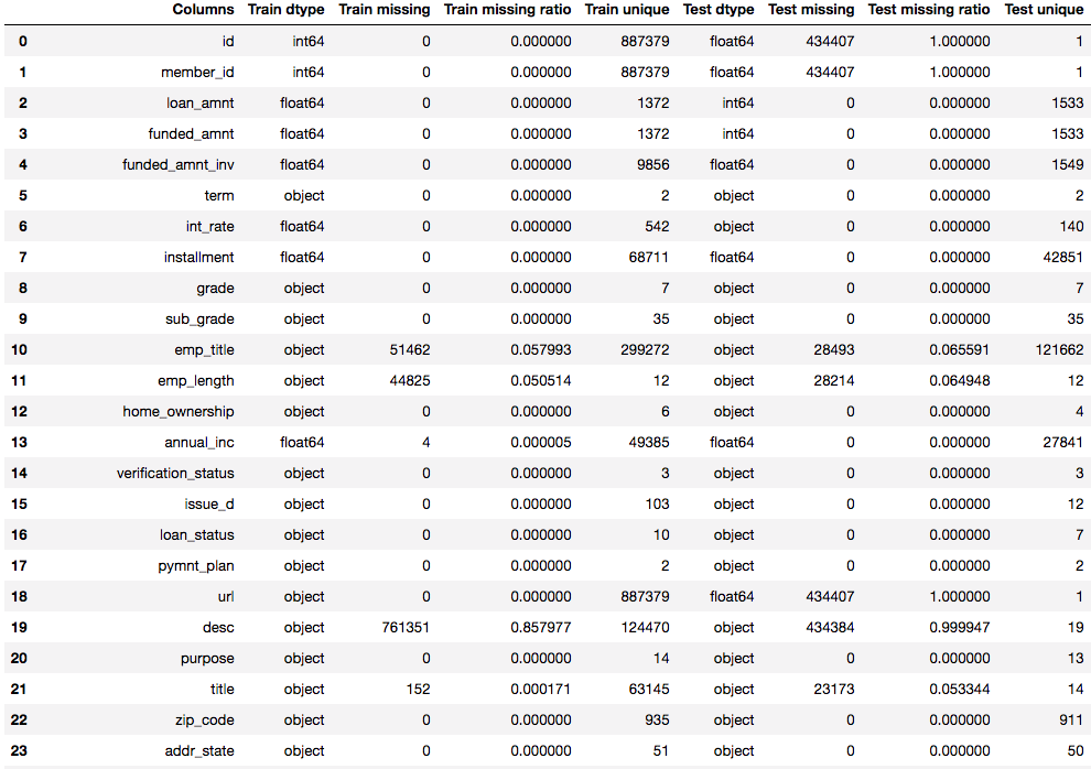
We should notice some differences between the training and test set, and look into details. Some major difference are:
- For test set, id, member_id, and url are totally missing, which is different from training set
- For training set, open_acc_6m, open_il_6m, open_il_12m, open_il_24m, mths_since_rcnt_il, total_bal_il, il_util, open_rv_12m, open_rv_24m, max_bal_bc, all_util, inq_fi, total_cu_tl, and inq_last_12m are almost missing in training set, which is different from test set
- desc, mths_since_last_delinq, mths_since_last_record, mths_since_last_major_derog, annual_inc_joint, dti_joint, and verification_status_joint have large amount of missing values
- There are multiple loan status, but we only concern whether or not the load is default
3. Data Cleaning and Initial Feature Engineering
Data cleaning and feature engineering are two of the most important steps. For this project, I have done the following parts.
I. Transform feature int_rate and revol_util in test set
II. Transform target values loan_status
In the training set, only 7% of all data have label 1. It’s clear that our dataset is highly imbalanced. (Note that here we treat current status also as label 0 to increase the difficulty. In other related projects, some people simply drop all the loan in current status. I have also explored that case, and you can easily get over 99% AUC on both training and test set even with logistic regression.)
III. Drop useless features
Now, we have successfully reduce the features from 74 to 40. Next, let’s focus on more detailed feature engineering First, let’s look at the data again. From the below table, we can see that:
- Most features are numerical, but there are severl categorical features.
- There are still some missing values among numerical and categorical features.
IV. Feature transformation
- Transform numerical values into categorical values
- Transform categorical values into numerical values (discrete)
V. Fill missing values
- For numerical features, use median
- For categorical features, use mode (here, we don’t have missing categorical values)
4. Visualization
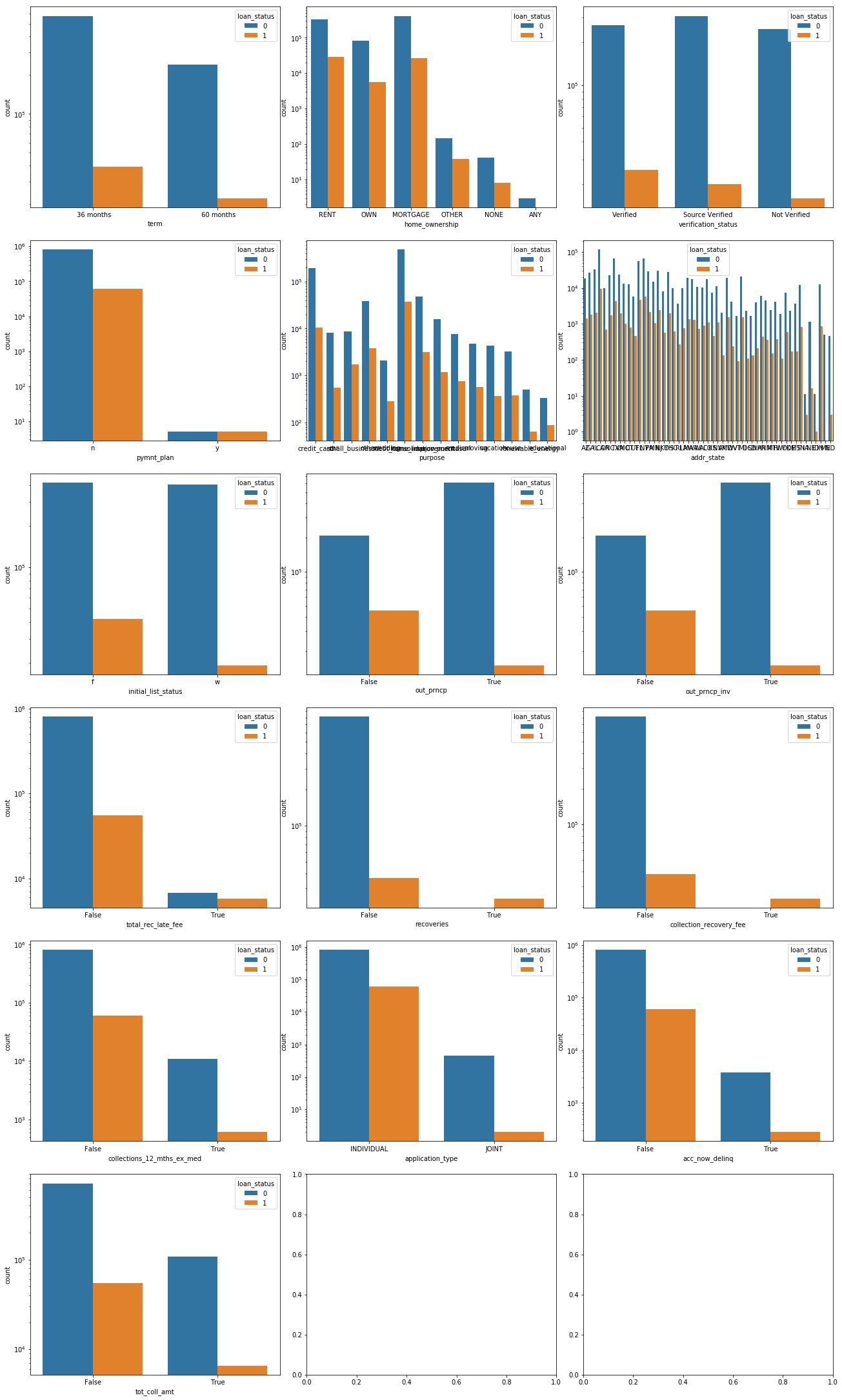
I. Visualize categorical features
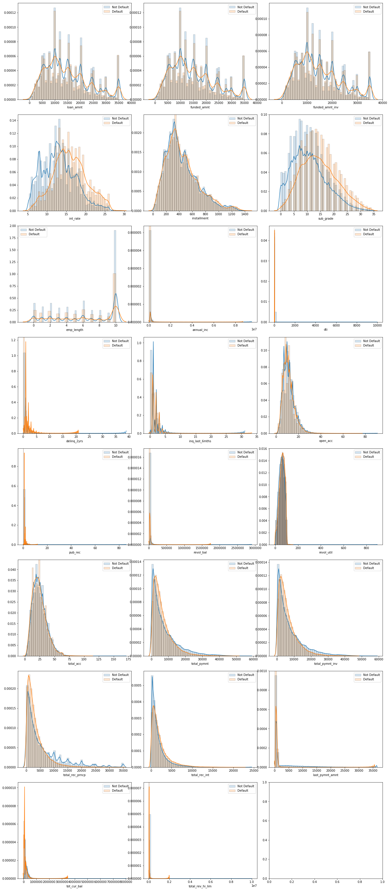
II. Visualize numerical features
5. Further Feature Engineering
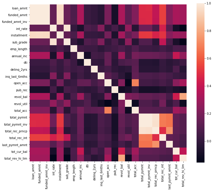
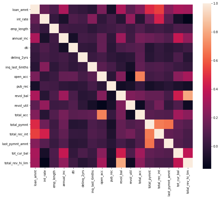
From the above heatmap and the categorical variable countplot, we can see that some feature has strong correlation
- loan_amnt, funded_amnt, funded_amnt_inv, installment
- int_rate, sub_grade
- total_pymnt, total_pymnt_inv, total_rec_prncp
- out_prncp, out_prncp_inv
- recoveries, collection_recovery_fee
We can drop some of them to reduce redundancy. Now, we only 14 categorical features, 17 numerical features. Let’s check the correlation again.
6. Machine Learning
After the above procedures, we are ready to build the predictive models. In this part, I explored three different models: Logistic regression, Random Forest, and Deep Learning.
I used to use scikit-learn a lot. But there is one problem with scikit-learn: you need to do one-hot encoding manually, which can sometimes dramatically increase the feature space. In this part, for logistic regression and random forest, I use H2O package, which has a better support with categorical features. For deep learning model, I use Keras with TensorFlow backend.
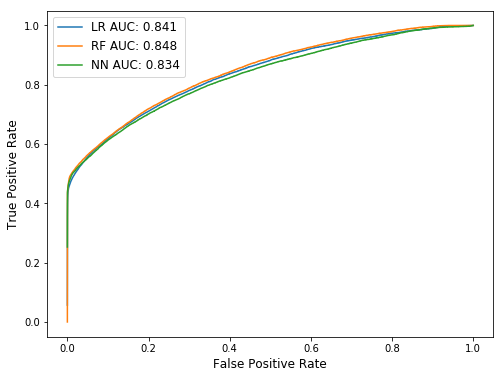
I. Logistic Regression
After grid search over alpha and lambda, I got test AUC of 0.841.
II. Random Forest
After grid search over alpha and lambda, I got test AUC of 0.848.
Feature Importance
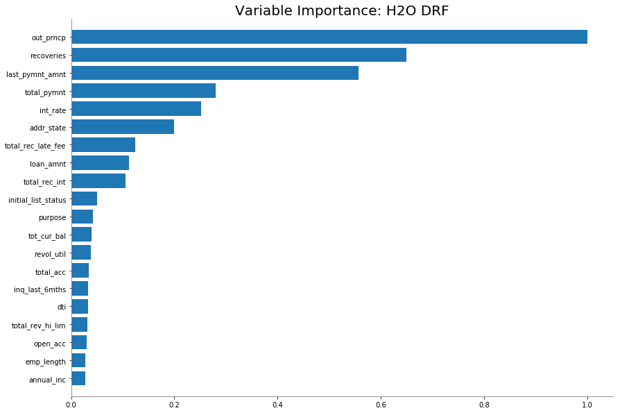
As shown above, the top 9 most important features are:
- out_prncp: Remaining outstanding principal for total amount funded
- recoveries: Post charge off gross recovery
- last_pymnt_amnt: Last total payment amount received
- total_pymnt: Payments received to date for total amount funded
- int_rate: Interest Rate on the loan
- addr_state: The state provided by the borrower in the loan application
- total_rec_late_fee: Late fees received to date
- loan_amnt: The listed amount of the loan applied for by the borrower. If at some point in time, the credit department reduces the loan amount, then it will be reflected in this value.
- total_rec_int: Interest received to date
III. Neural Networks
In this part, let’s manually build a fully-connected neural network (NN) model to finish the classification task. I use a relatively small model with only two hidden layers. Without comprehensive parameter tuning, the model gives AUC of 0.834.
7. Conclusions
From our above analysis, we can see that for the above three algorithms: Logistic Regression, Random Forest, and Neural Networks, their performance on the test set is pretty similar. Based on our simple analysis and grid search, Random Forest gives the best result.
There are a lot of other methods, such as AdaBoost and XGBoost, and we can tune a lot of parameters for different models, especially for Neural Networks. Here, I didn’t explore all possible algorithms and conduct comprehensive parameter tune. For more details, please refer to my GitHub jupyter notebook.
Footnote:
In this project, to increase the problem difficulty, the loan with status like “current” is treated as status 0, which might not be very appropriate. There are some other online analysis that exclude all the loan that is still in “current” status. I also conducted analysis with that kind of dataset, which is less imbalanced. I can easily get over 0.99 AUC on both training and test dataset even with simple logistic regression. You can try it by yourself if interested.